R Basics

Starting R (or your IDE)

Example of a R startup message:

R version 3.5.1 (2018-07-02) -- "Feather Spray"
Copyright (C) 2018 The R Foundation for Statistical Computing
Platform: x86_64-redhat-linux-gnu (64-bit)

R is free software and comes with ABSOLUTELY NO WARRANTY.
You are welcome to redistribute it under certain conditions.
Type 'license()' or 'licence()' for distribution details.

  Natural language support but running in an English locale

R is a collaborative project with many contributors.
Type 'contributors()' for more information and
'citation()' on how to cite R or R packages in publications.

Type 'demo()' for some demos, 'help()' for on-line help, or
'help.start()' for an HTML browser interface to help.
Type 'q()' to quit R.

RStudio

Here just a really brief overview. After opening RStudio, the screen is split in multiple panes.

png

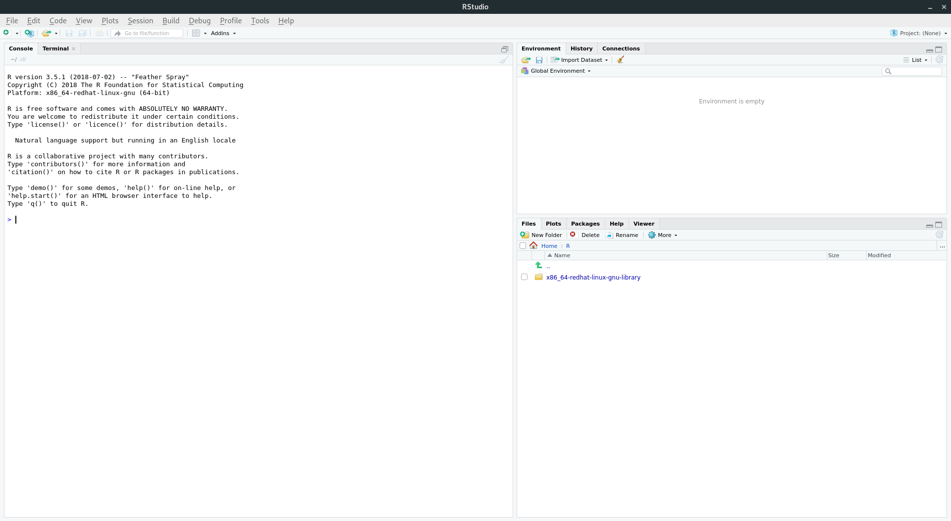
You will need to create a new script (green +, topleft). Topright is an environment overview, bottomleft the R console and bottomright the plot/help-window. Further materials on RStudio can be found here.

First Program

Depending on your IDE, you can write a script in your editor and then send it to R. A minimal version is to copy and paste scripts. The most important shortcut is ctrl+enter: run current line/selection. With this you can send your selected code directly to R. Working with R is highly interactive; you receive immediate feedback on your actions.

print("Hello World!")

Hello World!

Using Functions

R uses a lot of functions. Functions are indicated with brackets (). This is a rather common notation for programming languages.

Available datasets

What is convenient, is that R itself comes with datasets. This allows us to jump right into action without data import/export. As a sidenote, some packages provide datasets on their own. Here is a way to display all available (base) datasets:

ls("package:datasets")

'ability.cov'
'airmiles'
'AirPassengers'
'airquality'
'anscombe'
'attenu'
'attitude'
'austres'
'beaver1'
'beaver2'
'BJsales'
'BJsales.lead'
'BOD'
'cars'
'ChickWeight'
'chickwts'
'co2'
'CO2'
'crimtab'
'discoveries'
'DNase'
'esoph'
'euro'
'euro.cross'
'eurodist'
'EuStockMarkets'
'faithful'
'fdeaths'
'Formaldehyde'
'freeny'
'freeny.x'
'freeny.y'
'HairEyeColor'
'Harman23.cor'
'Harman74.cor'
'Indometh'
'infert'
'InsectSprays'
'iris'
'iris3'
'islands'
'JohnsonJohnson'
'LakeHuron'
'ldeaths'
'lh'
'LifeCycleSavings'
'Loblolly'
'longley'
'lynx'
'mdeaths'
'morley'
'mtcars'
'nhtemp'
'Nile'
'nottem'
'npk'
'occupationalStatus'
'Orange'
'OrchardSprays'
'PlantGrowth'
'precip'
'presidents'
'pressure'
'Puromycin'
'quakes'
'randu'
'rivers'
'rock'
'Seatbelts'
'sleep'
'stack.loss'
'stack.x'
'stackloss'
'state.abb'
'state.area'
'state.center'
'state.division'
'state.name'
'state.region'
'state.x77'
'sunspot.month'
'sunspot.year'
'sunspots'
'swiss'
'Theoph'
'Titanic'
'ToothGrowth'
'treering'
'trees'
'UCBAdmissions'
'UKDriverDeaths'
'UKgas'
'USAccDeaths'
'USArrests'
'UScitiesD'
'USJudgeRatings'
'USPersonalExpenditure'
'uspop'
'VADeaths'
'volcano'
'warpbreaks'
'women'
'WorldPhones'
'WWWusage'

Let's select the Theoph dataset. It is data about asthma medication. By applying the help function, more information is available. For brevity, this is not included here. help(Theoph)

A good first glance on new data sets is the head function. Per default, it shows the first five rows.

head(Theoph)

Subject	Wt	Dose	Time	conc
1	79.6	4.02	0.00	0.74
1	79.6	4.02	0.25	2.84
1	79.6	4.02	0.57	6.57
1	79.6	4.02	1.12	10.50
1	79.6	4.02	2.02	9.66
1	79.6	4.02	3.82	8.58

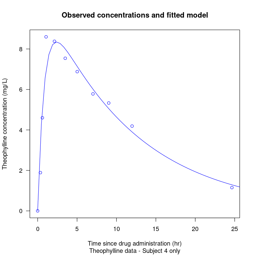
As shown in Lesson 1, a demo is available for the dataset Theoph. No need to understand details here.

# Demo from help(Theoph)
require(stats); require(graphics)

coplot(conc ~ Time | Subject, data = Theoph, show.given = FALSE)
Theoph.4 <- subset(Theoph, Subject == 4)
fm1 <- nls(conc ~ SSfol(Dose, Time, lKe, lKa, lCl),
           data = Theoph.4)
# summary(fm1)

plot(conc ~ Time, data = Theoph.4,
     xlab = "Time since drug administration (hr)",
     ylab = "Theophylline concentration (mg/L)",
     main = "Observed concentrations and fitted model",
     sub  = "Theophylline data - Subject 4 only",
     las = 1, col = 4)
xvals <- seq(0, par("usr")[2], length.out = 55)
lines(xvals, predict(fm1, newdata = list(Time = xvals)),
      col = 4)

png

Brief Introduction to Functions

Functions are fundamental in R. Without functions, readability and code re-usage and distribution, etc. would be vastly hindered. Typically functions look like this: function(param1). The variable param1 is an argument of the function, which is given to the function. With this argument the function does something:

print("A") # The print function prints the letter "A" to the command line.

[1] "A"

It is also possible to have multiple parameters, if the function was designed accordingly:

data.frame("A", row.names="B") # The function data.frame has the argument row.names.

	X.A.
B	A

Use the help function.

In the R help, possible arguments for functions are usually listed.

It is also possible to provide no argument to a function.

ls() # no output though.

Basic operations

Calculations

(1 + 1 - 2) * 3 * 1e6 / 100 # +-*/

17 %/% 5 # whole number division

17 %% 2 # modulo operation: gives remainder. Useful for odd/even calculations.

5^2 # power

abs(-100) # absolute number

100

round(100.50,0) # Round function. Careful.

100

If you want a different behavior (0.5 -> 1), you can find something here. b

Assignments

It would be nice to store values:

save <- 1+1 # in R, usually the arrow is used for assignment instead of =, even though both are possible.

save # no need to use print. Just type the variable name.

Together with functions, assignments are already incredibly powerful. You can store values and do something with them.

ls() # with the ls() function, all available objects in your environment are displayed.

'save'

It is possible to delete or remove objects from your environment.

rm(save) # Here the variable is removed.

ls() # check: now it's gone.

However, in the common R-script having objects in memory is not an issue. My usual way to go is to clean and prepare data in a first step and export them. Then I would restart R to avoid issues with available functions or variable, start a new script and just import the data. Other ways would be to remove everything and append your script. Then it can be run all in a go. R is usually quite open to allow for a multitude of different ways. Unfortunately, because of this property it can be a bit overwhelming in the beginning.

That's it (for now)!

So far, after setting up the workspace, we scratched help and documentation, functions, calculations and assignment. Next we will see some data types.