R Administration
The goal of the tutorial is to provide a short introduction as well as a lookup of code examples for myself. I am familiar with R in Linux and Windows, so there will be focus on these 2 platforms.
Installation
Here you can get R.
You could write code only in R, but you do not have syntax highlighting nor can you save the script conveniently. That's why an external editor would be useful. Examples are found here. I personally use emacs.
Windows: I recommend RStudio.
Linux: Get whatever IDE (integrated development environment) you want and install R from command line. To use R in terminal just type "R".
Customizing
R-Studio provides a lot of options. Here are some examples for directly editing the Rprofile.site (see below): 1. Quick-R, 2. blog of tony fischetti.
Packages
It is easy to extended R with packages. In later lessons I will introduce a few of them. To install them use the function install.packages() in R.
For each session, you will be asked to provide a CRAN-mirror.
The Comprehensive R Archive Network has mirrors all over the world. Just pick one nearby.
Under Linux, packages installed via R are locally compiled, under Windows binaries are installed. In Linux, it is often possible to install binaries via the packaging manager of the distribution. Here some information for ubuntu and here for redhat-based distributions. Linux has requirements for building (and it takes longer), so installing new packages is actually easier under Windows.
Library installation folder
Best is to use the function .libPaths() inside R. If you have multiple entries, the first one is the default. If you want to change the installation folder, you best write a custom directory in the file Rprofile.site.
This file can be found in Windows under the installation folder/etc. In Linux the file .Rprofile can be edited in the home directory. Why would you want to do that? Per default, (at least in Linux) the libraries are saved in a folder under a specific R version. It would be easier for updates, if they were stored somewhere independent from the R-version.
Useful packages
install.packages(c("ggplot","ggthemes","dplyr","zoo","chron"))
Updating packages
update.packages()
Further Information
Help Sources (out of R)
If you stumble upon problems, or have specific questions, stack overflow is a good place to look. What is rather strong in R, are also the mailing lists, namely R-help. The help there is rather fast and there are many R-gurus around... If you ask, provide some minimal code examples, and read the guidelines beforehand, otherwise you might receive some snappy answers. Another option is Rdocumentation.
Help inside R
There are the functions help(abc) and ?(abc) or ?"abc" or ?abc. help() is a bit more verbose than ?(). Some packages come with a more exhaustive documentation (vignettes), which can be found with browseVignettes(). More details are to be found here.
A very convenient feature is, that usually package help contains some demo code. Also, some packages provide a demo. Running demo() shows all available demos from the loaded packages.
demo(nlm) demo(nlm)
---- ~~~
> # Copyright (C) 1997-2009, 2017 The R Core Team
>
> ### Helical Valley Function
> ### Page 362 Dennis + Schnabel
>
> require(stats); require(graphics); require(utils)
> theta <- function(x1,x2) (atan(x2/x1) + (if(x1 <= 0) pi else 0))/ (2*pi)
> ## but this is easier :
> theta <- function(x1,x2) atan2(x2, x1)/(2*pi)
> f <- function(x) {
+ f1 <- 10*(x[3] - 10*theta(x[1],x[2]))
+ f2 <- 10*(sqrt(x[1]^2+x[2]^2)-1)
+ f3 <- x[3]
+ return(f1^2 + f2^2 + f3^2)
+ }
> ## explore surface {at x3 = 0}
> x <- seq(-1, 2, length.out=50)
> y <- seq(-1, 1, length.out=50)
> z <- apply(as.matrix(expand.grid(x, y)), 1, function(x) f(c(x, 0)))
> contour(x, y, matrix(log10(z), 50, 50))
> str(nlm.f <- nlm(f, c(-1,0,0), hessian = TRUE))
List of 6
$ minimum : num 1.24e-14
$ estimate : num [1:3] 1.00 3.07e-09 -6.06e-09
$ gradient : num [1:3] -3.76e-07 3.49e-06 -2.20e-06
$ hessian : num [1:3, 1:3] 2.00e+02 -4.07e-02 9.77e-07 -4.07e-02 5.07e+02 ...
$ code : int 2
$ iterations: int 27
> points(rbind(nlm.f$estim[1:2]), col = "red", pch = 20)
> stopifnot(all.equal(nlm.f$estimate, c(1, 0, 0)))
> ### the Rosenbrock banana valley function
>
> fR <- function(x)
+ {
+ x1 <- x[1]; x2 <- x[2]
+ 100*(x2 - x1*x1)^2 + (1-x1)^2
+ }
> ## explore surface
> fx <- function(x)
+ { ## `vectorized' version of fR()
+ x1 <- x[,1]; x2 <- x[,2]
+ 100*(x2 - x1*x1)^2 + (1-x1)^2
+ }
> x <- seq(-2, 2, length.out=100)
> y <- seq(-0.5, 1.5, length.out=100)
> z <- fx(expand.grid(x, y))
> op <- par(mfrow = c(2,1), mar = 0.1 + c(3,3,0,0))
> contour(x, y, matrix(log10(z), length(x)))
> str(nlm.f2 <- nlm(fR, c(-1.2, 1), hessian = TRUE))
List of 6
$ minimum : num 3.97e-12
$ estimate : num [1:2] 1 1
$ gradient : num [1:2] -6.54e-07 3.34e-07
$ hessian : num [1:2, 1:2] 802 -400 -400 200
$ code : int 1
$ iterations: int 23
> points(rbind(nlm.f2$estim[1:2]), col = "red", pch = 20)
> ## Zoom in :
> rect(0.9, 0.9, 1.1, 1.1, border = "orange", lwd = 2)
> x <- y <- seq(0.9, 1.1, length.out=100)
> z <- fx(expand.grid(x, y))
> contour(x, y, matrix(log10(z), length(x)))
> mtext("zoomed in");box(col = "orange")

> points(rbind(nlm.f2$estim[1:2]), col = "red", pch = 20)

> par(op)

> with(nlm.f2,
+      stopifnot(all.equal(estimate, c(1,1), tol = 1e-5),
+                minimum < 1e-11, abs(gradient) < 1e-6, code %in% 1:2))

> fg <- function(x)
+ {
+     gr <- function(x1, x2)
+         c(-400*x1*(x2 - x1*x1)-2*(1-x1), 200*(x2 - x1*x1))
+     x1 <- x[1]; x2 <- x[2]
+     structure(100*(x2 - x1*x1)^2 + (1-x1)^2,
+               gradient = gr(x1, x2))
+ }

> nfg <- nlm(fg, c(-1.2, 1), hessian = TRUE)

> str(nfg)
List of 6
 $ minimum   : num 1.18e-20
 $ estimate  : num [1:2] 1 1
 $ gradient  : num [1:2] 2.58e-09 -1.20e-09
 $ hessian   : num [1:2, 1:2] 802 -400 -400 200
 $ code      : int 1
 $ iterations: int 24

> with(nfg,
+      stopifnot(minimum < 1e-17, all.equal(estimate, c(1,1)),
+                abs(gradient) < 1e-7, code %in% 1:2))

> ## or use deriv to find the derivatives
>
> fd <- deriv(~ 100*(x2 - x1*x1)^2 + (1-x1)^2, c("x1", "x2"))

> fdd <- function(x1, x2) {}

> body(fdd) <- fd

> nlfd <- nlm(function(x) fdd(x[1], x[2]), c(-1.2,1), hessian = TRUE)

> str(nlfd)
List of 6
 $ minimum   : num 1.18e-20
 $ estimate  : num [1:2] 1 1
 $ gradient  : num [1:2] 2.58e-09 -1.20e-09
 $ hessian   : num [1:2, 1:2] 802 -400 -400 200
 $ code      : int 1
 $ iterations: int 24

> with(nlfd,
+      stopifnot(minimum < 1e-17, all.equal(estimate, c(1,1)),
+                abs(gradient) < 1e-7, code %in% 1:2))

> fgh <- function(x)
+ {
+     gr <- function(x1, x2)
+         c(-400*x1*(x2 - x1*x1) - 2*(1-x1), 200*(x2 - x1*x1))
+     h <- function(x1, x2) {
+         a11 <- 2 - 400*x2 + 1200*x1*x1
+         a21 <- -400*x1
+         matrix(c(a11, a21, a21, 200), 2, 2)
+     }
+     x1 <- x[1]; x2 <- x[2]
+     structure(100*(x2 - x1*x1)^2 + (1-x1)^2,
+               gradient = gr(x1, x2),
+               hessian  =  h(x1, x2))
+ }

> nlfgh <- nlm(fgh, c(-1.2,1), hessian = TRUE)

> str(nlfgh)
List of 6
 $ minimum   : num 1.13e-17
 $ estimate  : num [1:2] 1 1
 $ gradient  : num [1:2] 1.30e-07 -6.56e-08
 $ hessian   : num [1:2, 1:2] 802 -400 -400 200
 $ code      : int 1
 $ iterations: int 24

> ## NB: This did _NOT_ converge for R version <= 3.4.0
> with(nlfgh,
+      stopifnot(minimum < 1e-15, # see 1.13e-17 .. slightly worse than above
+          all.equal(estimate, c(1,1), tol=9e-9), # see 1.236e-9
+          abs(gradient) < 7e-7, code %in% 1:2)) # g[1] = 1.3e-7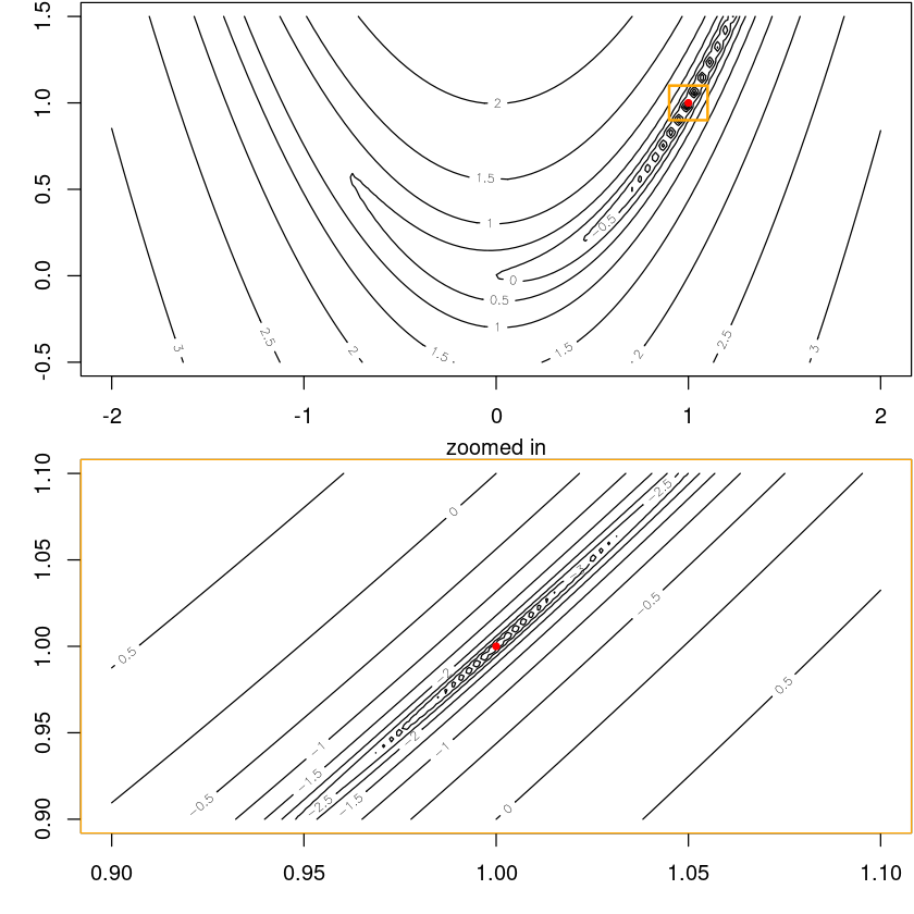
Literature
Literature about R: There are huge piles of books available. For instance, a list. For the German speaking world, I can recommend this book.
Courses
There are also courses available online, like from edX, or from datacamp. And maybe swirl.
Miscellaneous
Saving workspaces
Don't. Here is why, and here is how.
Updating R
Under windows, you basically can just download and install a new version. More convenient would be probably installr.
In Linux, newer versions automatically come via the package manager. There are also other options like building from source.
That's it (for now)!
After installing R and an appropriate IDE, setting up the package environment (optional), and adjusting R (or the IDE), we are ready to go further!